
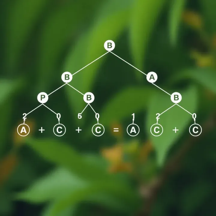
Understanding Binary Trees: Structure and Uses
Explore binary trees 🌳: their structure, types, traversal methods, and uses in programming. Understand operations and memory aspects for effective algorithm design.
Edited By
Henry Dawson
Binary trees form one of the most fundamental data structures in computer science, valued for their versatile applications in searching, sorting, and hierarchical data representation. Unlike general trees, a binary tree constrains each node to have at most two children: commonly called the left and right child. This clear structural limit shapes how information is stored and accessed efficiently.
To appreciate binary trees better, it helps to look beyond definitions and understand their structure and properties. For instance, consider node count and tree height. If a binary tree has a height h (where height is the longest path from root to leaf), then the maximum possible number of nodes is given by 2sup>h+1sup> - 1. This means a binary tree of height 3 can host up to 15 nodes at most. Such relationships guide developers when allocating memory or optimizing algorithms.

The configuration of nodes in a binary tree can vary widely. It may be a complete binary tree, where all levels except possibly the last are fully filled, and all nodes are as far left as possible. This arrangement is favoured in heap data structures. Alternatively, a perfect binary tree has all internal nodes with two children and all leaves at the same level, providing ideal balance for searching operations like in balanced binary search trees.
Understanding these forms is essential, as they directly affect traversal techniques (inorder, preorder, postorder), search efficiency, and storage methods.
Binary trees also follow constraints on nodes per level. Level zero (root) holds one node; level one can have up to two, level two up to four, doubling with each step down the tree. This exponential growth underpins many algorithms in computing and finance, such as decision trees used in trading algorithms to evaluate various market scenarios.
In practice, the height and balance of a binary tree influence performance. Unbalanced trees can degenerate into linked lists, making searches inefficient. Balancing methods (like AVL or Red-Black trees) maintain structural properties, ensuring logarithmic time complexity for insertion, deletion, and search.
In summary, grasping the basic structural limits, node configurations, and growth patterns of binary trees provides a strong foundation for utilising them effectively in data-driven applications across finance, technology, and education.
Understanding the fundamental structure of a binary tree sets the stage for grasping its practical applications in computing and data handling. A binary tree is a hierarchical data arrangement where each node links to at most two child nodes. This limitation of two children per node makes it different from other tree structures and is key to its efficient traversal and storage.
A tree becomes "binary" specifically because each node holds no more than two children, typically called the left and the right child. This conditional setup helps simplify many operations like searching, inserting, or deleting elements compared to more general trees with multiple children. For example, a binary search tree arranges elements so that the left child is smaller than the parent, and the right child is larger, allowing faster lookup times—something that is crucial in financial databases or trading algorithms where speed matters.
In a binary tree, a node represents a data point, such as a stock price or transaction record. Nodes connect with edges, which are the lines or links showing relationships between parent and child nodes. These connections form the tree’s backbone. Additionally, nodes are arranged in levels, with the root node at level zero. Each subsequent level consists of the children of nodes from the previous level. For instance, in a portfolio management system, the top level might represent different asset classes, with their associated stocks branching out on lower levels.
Each of these components determines how effectively the binary tree handles data operations, which directly impacts system performance in fast-paced environments like stock trading or risk analysis.
By defining these elements clearly, you gain insight into the binary tree's structure and its ability to organise data efficiently. This clarity aids in designing balanced trees, which optimise search times and resource use—vital factors when handling large volumes of real-time financial data or streaming updates from markets.

Understanding the different shapes and sizes of binary trees is vital, especially when dealing with algorithms and data structures. These variations directly affect the efficiency of operations like search, insert, and traversal, which traders and investors might relate to when handling large datasets or market trends. For example, a perfectly balanced tree enables faster search times compared to a skewed one, which can behave much like a linked list and slow down processing.
A full binary tree is one where every node has either zero or two children. This structure ensures no node has a single child, helping maintain balance. Consider a tournament bracket where every match pairs two competitors – this resembles a full binary tree.
A complete binary tree is slightly different; all levels are fully filled except possibly the last, which fills from left to right. This feature makes complete binary trees ideal for heaps in priority queues, widely used in financial applications that prioritise orders or transactions efficiently.
A perfect binary tree combines the properties of full and complete binary trees—all internal nodes have two children, and all leaves lie at the same level, producing a perfectly balanced tree. This type ensures the most efficient division of data and consistent performance in operations, making it valuable for balanced search trees.
In contrast, a degenerated binary tree looks more like a linked list, with each parent having only one child. This shape arises when the data is inserted in a sorted manner without self-balancing. For example, if you insert sorted stock prices into a binary search tree without balancing, the tree degrades and search operations slow down, which can hamper real-time analytics.
A skewed binary tree is a degenerated tree leaning entirely to the left or right. While simpler to implement, skewed trees perform poorly for searches, resembling sequential scans rather than efficient traversals. Traders and analysts need to be cautious about these structures since they can cause delayed information retrieval in time-sensitive decision-making.
Knowing these shapes helps in selecting or designing the right binary tree variant for your needs, whether it's maintaining balanced datasets or optimising quick lookups in financial software.
By grasping the nuances of these binary tree forms, you can better anticipate performance bottlenecks and tailor your data structures accordingly. Whether dealing with batch data processing or real-time streaming, picking the right binary tree shape can make a tangible difference in application speed and resource management.
Understanding the maximum number of nodes at each level is fundamental to grasping binary tree capacity and performance. Binary trees have distinct properties where each level can hold a limited number of nodes, which directly impacts how data structures manage space and retrieve information.
In a binary tree, the maximum nodes per level double as we move down from the root. The root level (level 0) has only one node. At level 1, the tree can hold at most 2 nodes, level 2 can have up to 4 nodes, level 3 up to 8, and so on. This pattern follows the formula:
math Maximum
For example, at level 4, the maximum nodes are 16 (2^4). This exponential growth reflects the binary nature where each node can have up to two children. However, in practical cases such as skewed or incomplete trees, this limit is often not met; many nodes may be missing.

> Remember, the maximum nodes per level help estimate the potential width of the tree, which influences memory allocation and traversal time.

### Calculating the Total Number of Nodes Based on Height

The total node count of a binary tree depends heavily on its height (the number of levels minus one). In a full binary tree where all levels are fully populated, the total nodes follow this formula:

```math
Total
Here, h is the height of the tree. Consider a binary tree of height 3; the total nodes would be:
2^4 - 1 = 16 - 1 = 15This means the tree can have up to 15 nodes if all levels except the last are completely filled.
In real-world scenarios like database indexing or computational parsing, fully complete trees are rare. Yet, understanding these limits guides optimisation and helps predict worst-case space requirements for binary search trees (BSTs) or heaps.
By combining knowledge of node limits at each level with the overall node count formula, you can better plan data structure size and performance. This is particularly critical when designing search algorithms or balancing techniques to maintain efficiency.
In short, knowing these maximums helps in assessing the space complexity and guides algorithm choices for tasks like sorting, searching, and hierarchical data representation.
Understanding the relationship between the height of a binary tree, its levels, and the number of nodes is fundamental to optimising its performance and structure. These factors determine how efficiently a tree can be traversed, searched, or modified. For traders and analysts dealing with hierarchical data or decision trees, appreciating this balance helps in selecting the right tree type and predicting performance overheads.
Height refers to the longest path from the root node down to a leaf. As height increases, the tree becomes taller, potentially heightening the number of levels. However, the ideal binary tree is balanced, keeping height to a minimum relative to the number of nodes. Unbalanced trees resemble linked lists, slowing down operations like search and insertion.
For example, a perfectly balanced binary tree with height h can have up to 2sup>h+1sup> - 1 nodes. This exponential growth means keeping height low results in efficient data organisation. If a tree with 31 nodes has height 4, it is balanced; but if the same nodes are arranged in skewed fashion, height could rise to 30, worsening search performance.
Balancing techniques, such as AVL or Red-Black trees, help maintain this equilibrium by restricting height changes during insertions or deletions, thus preserving efficient operations.
The height and node count directly influence traversal time and algorithm efficiency. Traversal methods—such as inorder, preorder, and postorder—are affected by how many levels must be navigated and how nodes are distributed.
In a balanced tree, operations like search, insert, or delete generally take O(log n) time, where n is the number of nodes. Conversely, an unbalanced, tall tree might degrade to O(n) time, similar to a linear list, which can cause delays in real-time processing or decision-making systems.
Traversal is also impacted by node placement. For example, if nodes cluster disproportionately on one side, algorithm stack usage increases due to deep recursive calls, stressing system memory.
Efficient tree structure means faster data access and less overhead in managing hierarchical data, which is crucial when handling large-scale financial datasets or complex computations.
In practice, recognising the interplay between these properties helps decide when to rebalance trees or consider alternative data structures. For instance, during market data analysis, swift updates and searches require a balanced tree to avoid computational lag.
Monitor tree height during dynamic insertions to identify imbalance early.
Use balancing algorithms to maintain optimal height.
Consider the nature of your data to choose tree types that suit traversal frequency and operation intensity.
This understanding equips developers and analysts alike to manage binary trees efficiently in environments demanding quick response and reliable data handling.
Explore binary trees 🌳: their structure, types, traversal methods, and uses in programming. Understand operations and memory aspects for effective algorithm design.

Learn binary search trees (BST) basics, operations like insertion, deletion, traversals, and their practical uses in software development. Perfect for Indian coders! 📚💻

Explore how optimal binary search trees ⚙️ boost search efficiency with practical examples, dynamic programming methods, and insights tailored for India 🇮🇳.
Explore how optimal binary search trees ⚙️ reduce search times efficiently. Learn key algorithms, structure, and real-world applications in data handling 📊.
Based on 11 reviews